Saturday, March 31, 2018

A family of fractal trees

Here is a new two-parameter family of fractal trees. The square of the width follows a Cantor function parameterised by the Cantor ratio c, which is 3/5 here:
the ratio c must be more than 0.5, with large values (here 0.75) giving wide, straight branches: 
and smaller values (here 0.52) giving thin, meandering branches:
The tree is built entirely from triangles which are all junction points. Here I show in white the largest of these triangles (c=0.525) which are all right-angled, making it a relative of the Pythagoras tree:

The right-angled triangles mean the tree obeys Leonardo's rule, maintaining total cross-sectional area if you assume a 3rd dimension for the branches. Like the Pythagoras tree, branches can overlap meaning the tree is immersed in (but not embedded in) 2D space. 

The branching is done by repeatedly splitting the length in half with alternating branching direction. Consequently a single branch is a relative of the Koch curve but with bend angle reducing towards the stem:
It is also possible to tweak the algorithm, for instance by flipping the direction of the offshoot branch:
however this gives very curly results, and I think of tweaks like this as non-standard variations of this tree family. 

The preserving of branch widths to power 2 is defined as the Pythagoras power p=2. But it doesn't have to be 2. "For real trees, the exponent in the equation that describes Leonardo's hypothesis is not always equal to 2 but rather varies between 1.8 and 2.3 depending on the geometry of the specific species of tree." Leonardo's rule
So p is the second adjustable parameter. If we reduce p to 1.4 we get:
making the triangles white we see that they are now less than 90 degree triangles:
Though they still tend to right angles triangles on the smallest offshoots compared to trunk width. 
We can reduce the width by reducing c (from 0.52) as it now can be less than half. Here we set it to 0.25:
Not only is the fork angle less when p is less than 2, but the small branches take up less proportion. Taken to the extreme we get an almost bare tree, (p=1.2, c=0.07):

As you can see, the tree width is affected by both c and p. It is easier to parameterise instead by the tree gradient and p. The gradient is: 
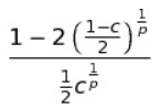
So c can be found to give the required gradient. Now a plot can be made of the 2D space of trees:
Here the triangle edges are drawn in grey. 

This 2D family has a number of sub-families of trees. There is of course the family of zero-area trees, which would sit just above the top row, with gradient=0. There is also the family of trees with symmetric central fork, I'll call these Cantor trees as they also use the exact one-third Cantor ratio c=1/3:
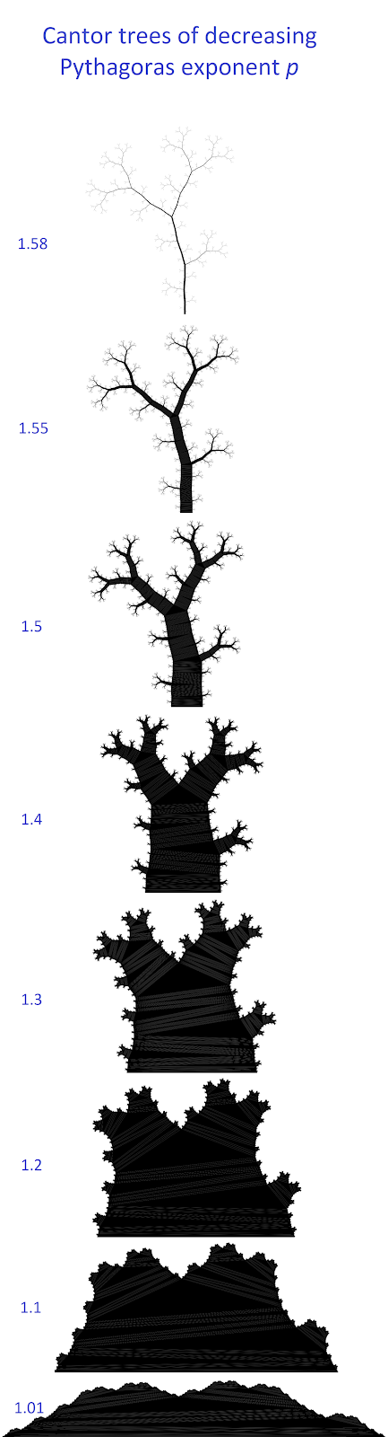
The intersection of these two sub-families is seen at the top of the above image. We might call this the Cantor fractal tree. 

So three sub-families are the thin (gradient 0) trees, the p=2 family (which we might call the Leonardo trees as they obey Leonardo's rule) and the Cantor trees above. A fourth subfamily is the family of balanced trees. These won't fall left or right. A property that is true of all their branches as well, if you pulled them off and stood them up. For low gradient trees the Pythagoras constant seems to be around 1.8:

Here is the family, the p values are approximate. Notice that the dominant branch moves from the left to the right branch as the tree gradient gets higher:

As such the balanced trees cross with the Cantor trees. The intersecting balanced Cantor tree has gradient of about 0.32:

Tuesday, March 27, 2018

Evolution in shapes

In my fractal classification I showed how scale-symmetric structures can be classified as a list and, for more expressive power, as a table. The base list is length 3, 5 and 7 for dimensions 1, 2 and 3. The first and last members are just nothing and solidness respectively and can be ignored as trivial cases. In addition the latter half of the list are negations of the opposite end of the list, where negation means emptiness and solidness are swapped. Consequently there are only 1, 2 and 3 unique shapes for dimensions 1, 2 and 3.

In that page I present a classification of moving structures, which is simply stating the range of classes in the above table or lists which the structure changes between during its lifetime. This has a lot of expressive power, but there is another, more constrained description for such dynamic fractals.

We can generalise the initial classification lists by giving them a time dimension. If the time dimension were like any other spatial dimension then the lists generalise easily. You would use the 3D list for the 2+1D case, and a 4D list for the 3+1D case. The 4D list has 9 elements, or 4 unique non-trivial elements.

anyway, time is different from other spatial dimensions. We can model it as having Lorentz rather than rotational symmetry, in which case the shapes are constrained to acting within light cones. The upshot of this is that (in the time direction) nothing grows to too sharp an angle, and objects don't suddenly appear from nothing. Other than this geometric constraint the list is the same for the +1 spatial dimension list.

So what does it look like?

In 1D we have intervals on the line which either grow from and to nothing, or continuously split.

The equivalent happens in 2D where we can have individual blobs growing and shrinking to nothing, and tree-like blobs that continually split into smaller trees and grow. We might call these two behaviours sporadic and asexual reproduction respectively.

There is a third behaviour in 2D, where network-like blobs split apart and change size, but eventually connect up with some other network-like blob. We might label this 'sexual reproduction' as the new child blobs always come from combined blobs.

The 'sexual reproduction' case is in some sense the special case in 2D, because geometrically it is the same class under negation. And 2D is the smallest dimension where it can happen. We note that most life on earth lives in a fairly 2D world due to the constraint of gravity.

However this is less the case in the ocean, and the 3+1D geometry contains a single new behaviour, which is the special case for 3+1D.

This behaviour looks like a 3D sponge (network of connected arms) where the arms split into two arms, thus making the network more complex, basically growing new mini versions of the network, and also growing in size overall. This behaviour is a little like the asexual case above, as it is unidirectional towards more complexity and growth, but it never separates and arms don't disconnect from their ends. So even though small versions of the network are continually generated and grown, there is no separation and the whole structure expands.

This is actually quite similar to the growth of a sea-sponge. The sea sponge is an unusual life form which many think of as a single organism but is in fact made of millions of unspecialised and quite independent cells.

Anyway it might be interesting to consider this third method of reproduction from an evolution standpoint, and whether it applies to sea sponges. Unlike asexual and sexual reproduction the genetic information is never detached, instead it could vary with location on the network, and the sub-network with effective variations might grow more than defective areas.

Another important area that evolves is the universe at large scales, and here there is perhaps an analogy to the sea sponge: Galaxy filaments and Galaxy walls (or sheets). Here the growth is from inflation and the formation into walls and then sheets is approximated by the Zeldovich pancake dynamics.

Saturday, March 24, 2018

Table of shapes by signed dimension

Here is a table of infinite extent shapes based on their signed-dimension. None of these structures have a Hausdorff or Minkowski dimension that lets them be measured. But the signed-dimension does.

Examples signed-D Type
-3 3D lattice
-2 3D graph
of edges
-2 2D lattice

-1 3D cell complex
of faces
-1 2D path
2D graph

1.26-2 Koch snowflake tiling

Grid of Cantor dust


0 infinite
   
1.13-1 chain of Gosper islands

2-1.63Tile based Sierpinski hexagon (yellow)
2-1.58 Cellular automata Sierpinski triangle

The Hausdorff and Minkowski formulae only consider the positive component of the dimension, resulting an an infinite measure on all unbounded structures.